When the user calculates the absorption or emission spectrum of a species using TDDFT, what the user obtains from the BDF program is a list of excitation energies and oscillator strengths in the .out file, for example (C60 molecule, PBE0/def2-SVP, first 10 T1u states):
  No. Pair   ExSym   ExEnergies  Wavelengths      f     D<S^2>          Dominant Excitations             IPA   Ova

    1 T1u    1 T1u    3.6161 eV    342.87 nm   0.0539   0.0000  79.2%  CV(0):  Hu(  26 )-> T1g(   7 )   4.228 0.724
    2 T1u    2 T1u    4.0346 eV    307.30 nm   0.5798   0.0000  58.7%  CV(0):  Hg(  46 )-> T1u(  19 )   4.396 0.707
    3 T1u    3 T1u    5.2174 eV    237.63 nm   2.4506   0.0000  63.5%  CV(0):  Hu(  26 )->  Hg(  51 )   5.475 0.693
    4 T1u    4 T1u    5.8548 eV    211.77 nm   0.0055   0.0000  85.7%  CV(0):  Hg(  41 )-> T1u(  19 )   6.866 0.566
    5 T1u    5 T1u    5.9297 eV    209.09 nm   0.0025   0.0000  72.1%  CV(0):  Hg(  46 )-> T2u(  19 )   6.749 0.746
    6 T1u    6 T1u    6.2930 eV    197.02 nm   3.3308   0.0000  62.5%  CV(0):  Fg(  21 )-> T2u(  19 )   6.724 0.706
    7 T1u    7 T1u    6.9435 eV    178.56 nm   0.0027   0.0000  85.6%  CV(0):  Hu(  21 )-> T1g(   7 )   7.789 0.539
    8 T1u    8 T1u    7.0070 eV    176.94 nm   1.0193   0.0000  87.4%  CV(0):  Hu(  26 )->  Fg(  25 )   7.751 0.662
    9 T1u    9 T1u    7.5243 eV    164.78 nm   0.0102   0.0000  91.5%  CV(0):  Hg(  36 )-> T1u(  19 )   8.351 0.645
   10 T1u   10 T1u    7.7409 eV    160.17 nm   0.0145   0.0000  75.0%  CV(0):  Hg(  46 )->  Hu(  31 )   8.596 0.599
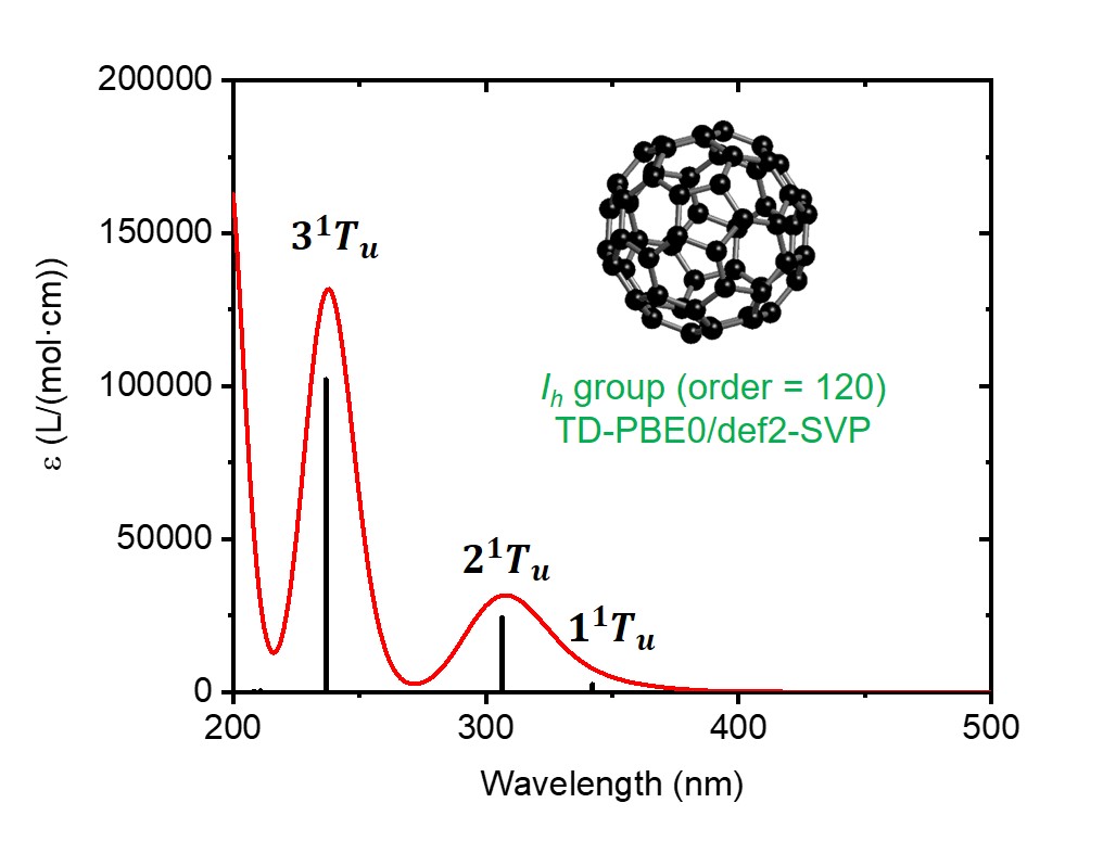
However, what the user really wants is frequently a continuous spectrum that properly reflects the non-zero widths of the peaks, similar to what is typically observed in experiments; the continuous spectrum is then usually plotted together with a set of vertical bars denoting the excitation energies and oscillator strengths of the excited states. This is what the tool plotspec.py (located under $BDFHOME/sbin/) is for. Given a .out file from a TDDFT job (e.g. C60.out), run
$BDFHOME/sbin/plotspec.py C60.out
or more simply
$BDFHOME/sbin/plotspec.py C60
The following information is printed to standard output:
==================================
      P  L  O  T  S  P  E  C

 Spectral broadening tool for BDF
==================================

BDF output file: C60.out

1 TDDFT output block(s) found
Block 1: 10 excited state(s)
 - Singlet absorption spectrum, spin-allowed

The spectra will be Gaussian-broadened (FWHM = 0.5000 eV) ...

Absorption maxima of spectrum 1 (nm (lg epsilon/(L/(mol cm)))):
 - 238 (5.12), 308 (4.50)

plotspec.py: exit successfully
The script generates two files. One of them is C60.stick.csv, which contains a list of wavelengths and extinction coefficients:
TDDFT Singlets 1,,
Wavelength,Extinction coefficient,
nm,L/(mol cm),
342.867139,2899.779319,
307.302300,31192.802393,
237.635960,131840.430395,
211.765024,295.895849,
209.090150,134.498113,
197.019205,179194.526059,
178.561512,145.257962,
176.943322,54837.570677,
164.778366,548.752301,
160.167663,780.089056,
The other is C60.spec.csv, which contains the Gaussian broadened spectrum (default FWHM=0.5eV):
TDDFT Singlets 1,,
Wavelength,Extinction coefficient,
nm,L/(mol cm),
200.000000,162720.545118,
201.000000,151036.824457,
202.000000,137429.257570,
...
998.000000,0.000000,
999.000000,0.000000,
1000.000000,0.000000,
One can then use the two files to plot the predicted absorption spectrum with e.g. Excel or Origin:

A few command line parameters can be specified to fine-tune the behavior of the script. Examples:
Plot the spectrum in the range 300-600 nm:
 $BDFHOME/sbin/plotspec.py wavelength=300-600nm filename.out

Plot an X-ray absorption spectrum in the range 200-210 eV, using a FWHM of 1 eV:
 $BDFHOME/sbin/plotspec.py energy=200-210eV fwhm=1eV filename.out

Plot a UV-Vis spectrum in the range 10000 cm-1 to 40000 cm-1, where the wavenumber is sampled at an interval of 50 cm-1:
 $BDFHOME/sbin/plotspec.py wavenumber=10000-40000cm-1 interval=50 filename.out

Plot an emission spectrum in the range 600-1200 nm, as would be given by Kasha's rule (i.e. only the first excited state is considered), where the wavelength is sampled at an interval of 5 nm:
 $BDFHOME/sbin/plotspec.py -emi wavelength=600-1200nm interval=5 filename.out
When the file filename.out contains the output of multiple TDDFT jobs (therefore multiple spectra), the spectra are plotted together, as different columns of the files filename.stick.csv and filename.spec.csv. For example, the .spec.csv file from a SOC-corrected transition metal L-edge X-ray absorption spectrum calculation may look like:
TDA Quartets 1,,TDA 6-tets 2,,TDA/TDDFT Spinors 3,,
Energy,Extinction coefficient,Energy,Extinction coefficient,Energy,Extinction coefficient,
eV,L/(mol cm),eV,L/(mol cm),eV,L/(mol cm),
576.000000,0.000000,576.000000,0.000000,576.000000,0.002005,
576.010000,0.000000,576.010000,0.000000,576.010000,0.002223,
576.020000,0.000000,576.020000,0.000000,576.020000,0.002464,
...
583.000000,2.611833,583.000000,0.000000,583.000000,122.580597,
583.010000,2.607841,583.010000,0.000000,583.010000,121.057743,
583.020000,2.610622,583.020000,0.000000,583.020000,119.510008,
...
591.980000,0.000000,591.980000,0.000000,591.980000,0.069449,
591.990000,0.000000,591.990000,0.000000,591.990000,0.063557,
592.000000,0.000000,592.000000,0.000000,592.000000,0.058133,
In this case the last column contains the SOC-corrected spectrum; the second column contains the spectrum without SOC correction (i.e. the spectrum from the first TDDFT block of the job).
For more detailed options, run $BDFHOME/sbin/plotspec.py without any command line parameter to show the full usage.